


The Dragonfly Project
An investigation into decoding Multi-Layer-Perceptrons (MLPs)


Introduction:
Recently, I began to wonder if Neural Networks, specifically Multi-Layer Perceptrons (MLPs), are all they are chalked up to be. I’d heard people describe MLPs as universal function approximators but questioned the notion of approximating functions if we could just use them. I figured, if nothing else, they may be a useful tool for the discovery of underlying equations in experimental data. So, in an effort to settle my curiosity, I set out on an adventure to decode model parameters and discover what makes the MLP special. I called it the Dragonfly project.1
After spending three months, making 400+ commits, and training over 120 models I figured it was time to share my results. To the experienced reader, some of these findings may be trivial but perhaps they are presented in a way that allows for novel insights.
I am making this post to begin a dialog on how the MLP architecture meshes with the natural world and how these models can become more interpretable.
From First Principals:
*If you know how an MLP works you can skip this section.
When I began this project the only thing I knew about neural networks was that they used a series of weighted sums that deterministically calculate a result. So, my first step was to understand their structure.

Frequently, neural networks are presented like the graphic above. But, at a high level, these models can simply be thought of as a series of interconnected pipes. You pour water down nodes X1, X2, and X3 and you get something out at the Y node. When someone says they are training a neural network all they are really doing is changing the size of these pipes to make the water flow faster or slower depending on what they want.
To gain a grasp of what is mathematically occurring with this pipe analogy let’s look at what happens between the three input nodes (X1, X2, and X3) and node A11.

The figure above, Figure 2, is a graphic of a perceptron which is the most simplified component of an MLP. This can be thought of as a function that takes in three inputs and outputs a single value. Mathematically, we can write this perception as the following function:
All that occurs here is the following:
Multiply each input value by a weight. (i.e. W[111])
Add all of them together.
Add a bias. (i.e. B[11])
If the outcome of step 3 is negative then your result is 0. Otherwise, the outcome of step 3 is your result. 2
From here, the same equation can be applied to solve for every other node until you arrive at your final value of Y. Through the model training process we are modifying the weight (i.e. W[111]) and bias values (i.e. B[11]) so our neural network aligns with our expected result.
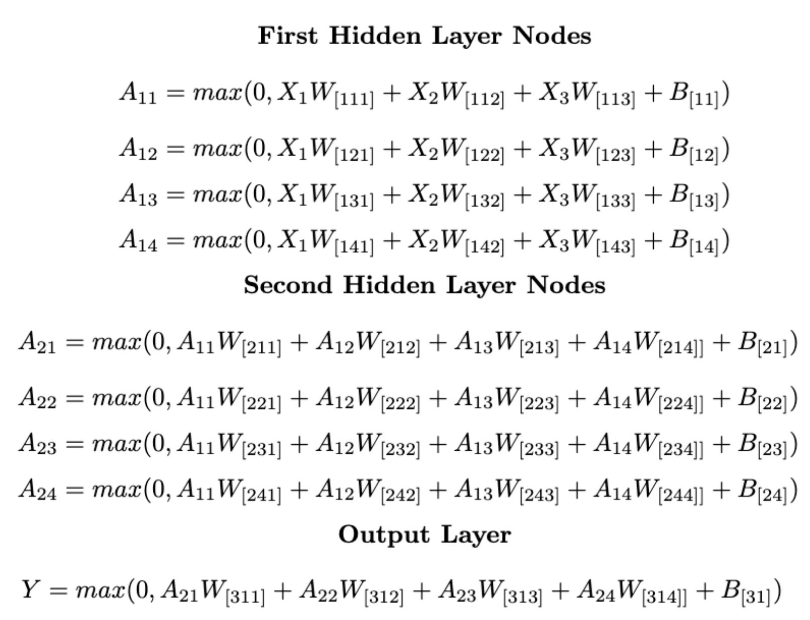
This entire process can be written as the series of equations above. I glossed over some nuances of the MLP model architecture. But, for the sake of this post, that’s the gist.
The Circumference Model:
A key tenant of this endeavor was to see if it is possible to come full circle on a trained neural network. This means I wanted to attempt to do the following:
Use an equation to generate model training data.
Use that training data to train an MLP.
Use the parameters of said MLP to “rediscover” the equation used to make the training data.
So… I tried to imagine what I would do if I had access to compute and the knowledge to train an MLP but lived in a world where we had yet to discover the equation for circumference.
As any great scientist, I would first start by generating a hypothesis. I may look at the coffee mug sitting on my desk and say “Hey” perhaps its height is related to its circumference. Or, maybe the diameter or rim thickness is correlated. So, I’d walk around and create a dataset of all the circular objects I find.
Object | Diameter(X1) | Height(X2) | Rim Thickness(X3) | Circumference |
------------------------------------------------------------------------
#1     |      7       |     4      |       0.08        |      21.9     |
#2     |      1       |     6      |       0.07        |      3.1      |
#3     |      3       |     1      |       0.12        |      9.4      |
#4     |      2       |     3      |       0.25        |      6.2      |
Once my data has been obtained, it is time to train a neural network to see if any of my hypotheses are correct. As you would expect, it's successful!
So, where do we stand?
The Pros:
We have experimental data that happens to include a key parameter. (Diameter - Lucky Guess!)
We have trained a Neural Network… and it works!
Now, anytime someone comes to us with the Diameter, Rim Thickness, and Height of an object we can use our neural network to solve for the circumference for them.
The Cons:
Our Neural Network is an incredibly inefficient way of solving for circumference.
We have no clue which parameters are actually correlated.
We gain no knowledge about fundamental constants that may exist. (π. - Ever heard of it? … No, not the dessert.)
Put simply, we have an inefficient solution that provides no insight or understanding. But, this is a pessimistic perspective. Perhaps we are closer to understanding how to compute circumference we just need to look elsewhere.
The Parameters:
Within our natural network exist 41 parameters that together can somehow compute the circumference of a circular object. If we were to look at them it doesn’t appear as if they would tell us much.
Here, take a look for yourself:

However, the equation identified by the MLP, which uses these weight and bias values, can be seen as a different form of the equation for circumference. Meaning, we could take parameters from Figure 4, plug them into the equations in Figure 3, and have an equation that exhibits near equality with the circumference equation. Therefore, these weight and bias values harbor the potential to unveil the circumference formula but also to allude to a deeper revelation: the constant π.
The Analysis:
The question becomes, how would we go about decoding this long equation from Figure 3 with parameters from Figure 4?
Fortunately, it turns out that every MLP can be rewritten as a single perception for each unique input. How? Well, you write out the entire MLP equation in terms of your input values and factor that equation to obtain a singular weight for each input and one bias value.
So, in an instance where our diameter == 1, circumference == 0, and rim thickness == 0, our neural network can be fully approximated as the following equation.
This process can be replicated for every other input value in our dataset to develop a granular view of how our neural network is calculating circumference. As a result, we get a model profile that looks like this:

From here, we can start to draw some conclusions about how circumference can be calculated.
First, we can see that the inputs X2 (Height) and X3 (Rim Thickness) have zero correlation to the circumference. This can be seen by the graph in Figure 4 and further cemented by the mean and standard deviation of the parameters.
Second, we can see that X1 (Diameter) is being multiplied by a constant value around 3.1. It becomes clear that this model is converging to a solution for circumference that just so happens to be equal to the equation we know.
Our model will converge to the equation:
Which just so happens to look a lot like:
In the unlikely scenario where we didn't know the equation for circumference but had access to MLPs, we could have used them to identify π and derive the circumference equation.
Fingerprinting:
At this point, I became curious to learn how other sorts of functions could be profiled so I set out to train more models and take a look.

In a not-so-surprising manner, it turned out that each function type had a clear and distinguishable profile that could be used to map to the original equation. Furthermore, this profiling could be done without looking at the input data but instead at the model’s parameters.
I was able to see that the profiles for inputs raised to even powers took the same shape at different scales. The same could be said of odd powers and even square roots.
My first thought was, ok, maybe if I generate enough of these profiles it would allow me to create a database of model-profile to functions mappings. If so, this analysis process could be helpful in three ways.
It would allow for an efficient feedback loop to see which model inputs are correlated. ← This could improve training.
It would allow for models to be much faster in inference. ← Why use a function approximator when you could use the function?
It would be a new tool to discover unknown equations and constants from experimental data. ← Could maybe help with new scientific discoveries. Neat.
Putting the Cart Before the Horse:
With these results, my mind immediately went to use cases. I was most intrigued by the idea of equation discovery and knew I first needed to train accurate models on data that did not conform to known equations.
Around this time, OpenAI had just released its first set of videos from Sora, two of which caught my eye. Outputs from their diffusion model seemed to exhibit accurate-looking depictions of turbulent fluid dynamics. To date, due to the nonlinearity of the Navier-Stokes equations, no analytical solution for turbulent flow has been identified. Perhaps, Sora had discovered one and this analysis process could uncover it.
But, I quickly realized that I had almost no knowledge of diffusion models, and quite frankly still don't, so figured it was best to start elsewhere.

Over a few months, I ventured down many paths and attempted to train multiple models with pitiful results. My process was not very structured, but I selected use cases based on the following criteria: (1) the availability of easily accessible training data, and (2) the absence of a known equation describing the input data.
Now, these criteria, particularly #2, put me in a situation where the likelihood of successfully creating an accurate model was unlikely. But, the likelihood of success didn’t seem to be zero so it was certainly worth a shot.
First, I attempted to train a model on a chaotic dataset. The objective was to develop a model to predict the next cell of CA Rule 30 without the context of the three cells above it. Certainly no harm in trying, right?
This was followed by attempts at creating models to predict primes, the trajectory of financial markets, and lift coefficients of airfoils, among others. All failed attempts but interesting nonetheless.
Training all of these models was enjoyable but had its moments of frustration. The worst part was that my Dell Poweredge R510 server was heating up my apartment faster than my AC unit could handle. It was a sweltering few weeks.
The Problem:
By this point, I had recognized that I put the cart before the horse and needed to take a step back to reevaluate. I looked back at the simple model profiles I created in the beginning and decided I should try to train a model where two inputs interact. Therefore, I settled on creating a simple multiplication model.
Overfitting was going to be a guarantee because the equation for a perceptron only relates two inputs through addition. But, I wanted to see what the model profile would look like for an overfit model that was essentially memorizing examples.
I was curious to know if there were some patterns I could identify through the model profiling process and hoped it would be memorizing inputs in a unique way. Maybe even a way that could shed light on a new approach for integer factorization.
The training took a while and the model was overfit as hell but it provided me with an insight I should have reached months ago. All I needed to see was the model profile.

After looking at Figure 8, I realized an MLP will not be able to approximate any mathematical operation where the input variables interact through anything other than addition/subtraction unless the model memorizes the input data.
My Conclusions:
So, where does this leave me?
As of today, I feel there is value in treating an MLP as a single perceptron for each unique input to analyze the model’s parameters. If nothing else, it allows for quick iteration on model development as non-correlated inputs become exposed. Furthermore, I suspect there are some instances where MLPs have been deployed and inference could be made more efficient by parameter function identification.
As for how this model architecture meshes with the natural world, I believe there is much to be desired. Take Newton’s law of universal gravitation for example.
You would be hard-pressed to get an MLP to approximate this function without only overfitting. Functions like these frequently present themselves in the natural world and I suspect our model architectures should accommodate them.
At the end of the day, great scientific advancements arise when discernible patterns emerge from experimental data. If our models can't align with that data without overfitting, we must innovate with new architectures.
Even so, some of the great models we have today may harbor important truths about the natural world hidden in long lists of floating-point numbers. Only by looking, with curiosity and determination, can we hope to uncover them.
Reflection:
Next, I will likely focus on exploring three different things:
Existing model architectures that can accommodate a larger range of function types.
New model architectures that can accommodate a larger range of function types.
Permutations that can be made to input data that would allow current MLP configurations to approximate function with variables that interact through operations other than addition.
As someone who has very little experience in the ML space, this project has been a blast. It hasn’t been without its challenges or frustrations but every second has been worth it.
All thoughts, recommendations, corrections, and questions are appreciated.
If you made it this far, thank you for reading! I enjoyed creating my first post on substack and hope you enjoyed reading it.
Why? IDK, it was just the name of an empty repo I had up on GitHub.
In this example, ReLU is used as the activation function.